Jack’s Car Rental
One of my goals this year is to learn more about reinforcement learning. To this end, I’ve been reading through Reinforcement Learning: An Introduction by Sutton and Barto, and working through the exercises. This post details a particular example from the book, and the algorithm used to solve it. I provide the output of the code I used to replicate the results, and some comments on the problem and the solution.
Problem Statement
From Sutton and Barto, p. 81:
Jack manages two locations for a nationwide car rental company. Each day, some number of customers arrive at each location to rent cars. If Jack has a car available, he rents it out and is credited 10 dollars by the national company. If he is out of cars at that location, then the business is lost. Cars become available for renting the day after they are returned. To help ensure that cars are available where they are needed, Jack can move them between the two locations overnight, at a cost of 2 dollars per car moved. We assume that the number of cars requested and returned at each location are Poisson random variables, meaning that the probability that the number is n is $\frac{\lambda^n}{n!}e^{-\lambda}$, where $\lambda$ is the expected number. Suppose $\lambda$ is 3 and 4 for rental requests at the first and second locations and 3 and 2 for returns. To simplify the problem slightly, we assume that there can be no more than 20 cars at each location (any additional cars are returned to the nationwide company, and thus disappear from the problem) and a maximum of five cars can be moved from one location to the other in one night. We take the discount rate to be $\gamma = 0.9$ and consider the problem of finding the optimal policy for maximizing the expected total reward.
The state is the number of cars at each location. The action is the number of cars to move from one location to the other. The reward is the profit from renting cars minus the cost of moving cars.
We identify the optimal policy using the policy iteration algorithm. We shall begin by reviewing the algorithm.
Policy Iteration Algorithm
Letting $\pi(a \mid s)$ denote the probability of taking action $a$ in state $s$ under policy $\pi$, the state-value function $v_{\pi}(s)$ is the expected return starting from state $s$, and then following policy $\pi$. That is,
\[v_{\pi}(s) = \mathbb{E}_{\pi}[G_t | S_t = s],\]where $G_t = R_{t+1} + \gamma R_{t+2} + \gamma^2 R_{t+3} + \ldots$ is the return, $R_k$ is the reward at time $k$, and $\gamma$ is the discount factor. Discounting is used to ensure that the return is finite, and to give more weight to immediate rewards. However, the particular value of $\gamma$ is arbitrary and must be specified in advance.
Letting $p(s’, r | s, a)$ denote the probability of transitioning to state $s’$ and receiving reward $r$ given that we are in state $s$ and take action $a$, and letting $\gamma$ denote the discount factor, the Bellman Equation states:
\[v_{\pi}(s) = \sum_{a} \pi(a|s) \sum_{s', r} p(s', r|s, a)[r + \gamma v_{\pi}(s')]\]which expresses the value of any state $s$ in terms of the expected value of the next state $s’$ and the expected reward $r$.
Provided a policy $\pi$, we can convert this into an iterative algorithm to find the corresponding value function, $v_{\pi}$. We start with an initial guess (e.g., $v_{\pi}^0 = \mathbf{0}$), and then repeatedly apply the Bellman Equation to each state until the value function converges. Explicitly, starting from $n=0$ we compute
\[v_{\pi}^{n+1}(s) = \sum_{a} \pi(a|s) \sum_{s', r} p(s', r|s, a)[r + \gamma v_{\pi}^n(s')]\]until $\max_s \lvert v_{\pi}^{n+1}(s) - v_{\pi}^n(s) \rvert < \theta$ for some small $\theta$. This is called iterative policy evaluation, as it evaluates the value of the policy at each state.
Once we have the value function $v_{\pi}$, we can use it to improve the policy by acting greedily with respect to it. Explicitly, we can define a new policy $\pi’$ such that $\pi’(s) = \arg\max_a \sum_{s’, r} p(s’, r \mid s, a)[r + \gamma v_{\pi}(s’)]$. This is called policy improvement. This new policy is guaranteed to be as good as or better than the old policy (with respect to the value function $v_{\pi}$).
We can then iterate between policy evaluation and policy improvement until the policy converges. This is called policy iteration. The pseudocode is as follows:
- Initialize $\pi$ arbitrarily
- Repeat until policy converges:
- Policy Evaluation:
- Initialize $v_{\pi}^0 = \mathbf{0}$ (or some other initial guess)
- Repeat until $\lvert v_{\pi}^{n+1}(s) - v_{\pi}^n(s) \rvert < \theta$ for all $s$:
- For each $s$:
- $v_{\pi}^{n+1}(s) = \sum_{a} \pi(a \mid s) \sum_{s’, r} p(s’, r \mid s, a)[r + \gamma v_{\pi}^n(s’)]$
- For each $s$:
- Policy Improvement:
- For each $s$:
- $\pi’(s) = \arg\max_a \sum_{s’, r} p(s’, r \mid s, a)[r + \gamma v_{\pi}(s’)]$
- If $\pi’ = \pi$, then stop, policy has converged.
- $\pi = \pi’$
- For each $s$:
- Policy Evaluation:
Results
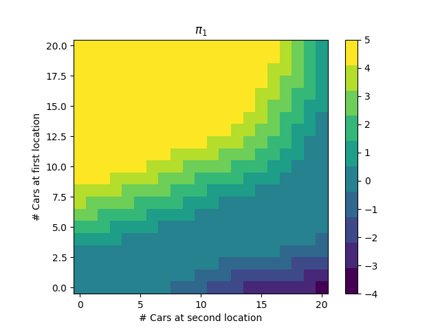
Starting from a policy that never moves cars ($\pi = \mathbf{0}$), the convergence of the first round of policy evaluation looks like the following:
Naturally, it’s better to have more cars available. After policy improvement, we get the new policy:
We then repeat the process, until we get the optimal policy:
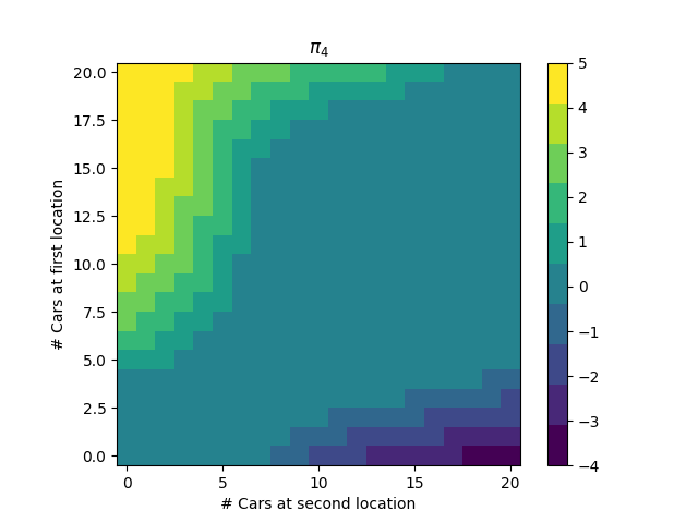
This policy passes a sanity check: it is better to move cars from location 1 to location 2 when there are much more cars at location 1 than location 2, and vice versa. Furthermore, location 1 and 2 are natural “sink” and “source” locations, respectively, as the expected number of cars requested at location 1 is lower than the expected number of cars requested at location 2, and the expected number of cars returned at location 1 is higher than the expected number of cars returned at location 2. Thus, we are more likely to have a surplus of cars at location 1, and a deficit of cars at location 2, and the policy reflects this.
Code
The code is available in this notebook.
Comments
- This is a “model-based” approach, as we need to know the transition probabilities $p(s’, r \mid s, a)$ to solve the problem. These values may be unknown or too multitudinous to compute in practice. Indeed, even in this toy problem, the most expensive step was construction of this table. For this reason, much of the book is devoted to “model-free” approaches, which do not require knowledge of the transition probabilities.
- Silent bugs are easy to introduce in this problem.
- There are subtle ambiguities in the problem statement. For example, while it is clear that the number of cars after a moving, renting, and returning iteration is clipped to 20, it is not clear if this value is limited after moving but before renting / returning. Indeed, in the second plot on p. 81 of Sutton and Barto, the policy says to move one car from location 1 to location 2 when there are 20 cars at both locations, which would mean 21 cars would be at location 2 after the move.