Good Turing Smoothing
I recently completed the Johns Hopkins Data Science Specialization with Coursera. The capstone project involves developing a text prediction model (you can find the app I created here). In this post, I’d like to describe an approach for text prediction I learned about while developing my algorithm.
The aim is to create an application that takes in some user-entered text, and produces a prediction for what the next word is going to be. For instance, the user could type in “Friends, Romans, countrymen, lend me your”, and the application might suggest “ears” (or, “hand” or “car” or whatever).
The approach that text prediction models use is to imagine a probability distribution over all possible words, given a sequence of input words. For example, if the input words are “lend me your”, then perhaps the probability of “ears” is 90%, and the probability of “cat” is 10%, and the probability of all other words is 0% (the sum of the probabilities over all the words has to be 100% for it to be a probability distribution).
Let’s put this in math terms. Let $w_i$ denote the next word in the sequence (that is, the one we wish to predict), and let $w_{i-1}$ be the previous word, and $w_{i-2}$ the word before that, and so on ($w_0$ would be the word at the beginning of the user-entered text. So, in our example, $w_{i-1}$ is “your”, $w_{i-2}$ is “me”, and $w_{i-3}$ is “lend”. Then, we are searching for the word $w_i$ that maximizes the conditional probability:
\[P(w_i \mid w_0w_1\dots w_{i-1})\]So, “all” we need to do is calculate this conditional probability for every word ever. Then, we select the word with the greatest conditional probability as our prediction.
In most text prediction models, we start with some large source of text data called a corpus. For instance, we can use the complete works of Shakespeare. We then use the text in that corpus to develop our model. Our algorithm will, hopefully, predict words in such a way that the resulting text sounds “Shakespearean”, even if the specific text itself never appears in Shakespeare.
How can we use a corpus to determine the probability of a word, given a sequence of previous words? Consider calculating the probability of “head” given the input “off with his”. A natural way to do is to simply count the number of times the phrase “off with his head” appears in the corpus, and divide that by the number of times “off with his” appears, i.e.:
\[P(\text{head} \mid \text{off with his}) \approx \frac{\text{Count}(\text{off with his head})}{\text{Count}(\text{off with his})}\]Apparently, “off with his” appears four times in Shakespeare:
## [1]"  QUEEN MARGARET. Off with his head, and set it on York gates;"
## [2] "    For Somerset, off with his guilty head."
## [3] "    Off with his head! Now by Saint Paul I swear"
## [4] "  KING RICHARD. Off with his son George's head!"
In two of them, the next word is “head”, but in one it’s “guilty” and in another it’s “son” (they’re all getting at the same idea, of course). We can then approximate the probability distribution of the words following “off with his” by saying there’s a 50% chance it’ll be “head”, a 25% chance of “guilty”, a 25% chance of “son”, and a 0% chance of every other word ever to exist, i.e.,
\[P(w_i \mid \text{off with his}) = \begin{cases} 0.5 & w_i = \text{head} \\ 0.25 & w_i = \text{guilty} \\ 0.25 & w_i = \text{son} \\ 0 & \text{otherwise} \end{cases}\]To approximate the probabilities in this way is to use the Maximum Likelihood Estimate, which is to use the probability distribution which best matches the observed data. We can already see the issue with the approach. Our model completely rules out words it’s never seen after “off with his”. However, it’s a pretty good starting point; this kind of model will predict “head” when a user types “off with his”.
There’s another issue here. For many input phrases, there won’t be any instances from which to estimate probabilities. For instance, the phrase “i can’t afford a hundred thousand” never shows up! We can’t assign probabilities to any word, let alone make a prediction for the next word. However, the phrase “a hundred thousand” shows up nine times:
## [1] "  MENENIUS. A hundred thousand welcomes. I could weep"
## [2] "    And I will die a hundred thousand deaths"
## [3] "  King. A hundred thousand rebels die in this!"
## [4] "     Shall break into a hundred thousand flaws"
## [5] "    The payment of a hundred thousand crowns;"
## [6] "    A hundred thousand more, in surety of the which,"
## [7] "    A hundred thousand crowns; and not demands,"
## [8] "    On payment of a hundred thousand crowns,"
## [9] "    As it should pierce a hundred thousand hearts;"
and, in three of the nine instances, the next word is “crowns”. For the other instances, the resulting sequence is the only time the phrase appears in the corpus. So, it might be reasonable to predict “crowns” as the next word.
We can observe the trade-off here. The more words in the input, the less likely it is that we’ll possess reliable data with which to calculate our predictions. Meanwhile, if we have fewer words in the input, there are more instances to work with, but they may not match our meaning as well (it doesn’t seem likely someone would say they can’t afford a hundred thousand welcomes, unless they’re explaining why they can’t be a hotel clerk).
When we use the probabilities generated by only looking at the most recent words, we’re making the following assumption:
\(P(w_i \mid w_0w_1\dots w_{i-1}) = P(w_i \mid w_{i-n+1}\dots w_{i-1})\) where $n$ is some positive integer. That is, we assume the probability of word $w_i$, given the input text, is only dependent on the most recent $n$ words. This is called a Markov assumption (an assumption of “memorylessness”); our probabilities completely ignore the earlier words in the text. For instance, if $n=2$, then we are saying the probability of observing $w_i$ only depends on the previous word, $w_{i-1}$, and when $n=3$, it only depends on the two most recent words: $w_{i-1}$ and $w_{i-2}$. We call these models “n-gram” models. When using $n=2$, we call it a bigram model, and when $n=3$, a trigram model.
Suppose we’re using a trigram model. That is, our prediction for the next word is going to be word $w_i$ that maximizes: \(P(w_i \mid w_{i-2}w_{i-1})\) We can estimate these probabilities by just looking at the counts:
\[P(w_i \mid w_{i-2}, w_{i-1}) = \frac{\text{Count}(w_{i-2}w_{i-1}w_i)}{\text{Count}(w_{i-2}w_{i-1})}\]For instance, predicting the next word in the phrase “have to”, we could look at all the sequences of three words (trigrams) starting with “have to”, count the instances for each, and divide each by the instances of the bigram “have to”. We can then produce the following plot of the five most probable words (as estimated by the trigram model):
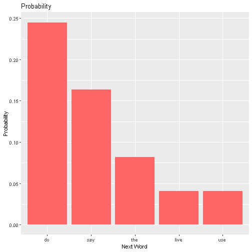 and observe “do” is the most likely candidate. We can use a similar process for larger $n$-grams. As discussed above, we need to keep in mind the trade-off between supplied information and data availability.
Suppose we have a trigram model, and we want to find the probability of the next word after “have to” being “run”. The phrase “have to run” never shows up, so our trigram model gives it a probability of zero. However, this doesn’t seem reasonable. Indeed, the phrase “to run” appears 14 times, so, given the verb is used by Shakespeare’s characters, it seems possible that a new Shakespearean character would want to describe their obligation to run.
Suppose we have a trigram model and a bigram model. If we had an enormous corpus, the former would almost certainly be a better predictor, since it has more context. However, with a limited corpus size, the trigram model has insufficient data to create a prediction (i.e., when the trigram never appears in the corpus). Meanwhile, the bigram model will have much more data, and it will often be the case that though a trigram doesn’t appear, the bigram consisting of the latter two words does. This motivates the following scheme: use the trigram probability if we can, and if not, use the bigram probability.
Back-off and Smoothing
This is known as a “back-off” model, where the “backing off” is us retreating from a trigram model to a less ambitious bigram model. Suppose we are using the back-off model, and the input phrase is “get thee”. Looking at the counts of all the words after “get thee”:
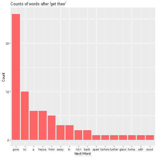
we see that “gone” appears 26 times, “to” 10 times, and so on (the word “<s>” refers to the end of the sentence.) In total, we have 16 unique choices that appear in Shakespeare. The trigram model would produce a probability distribution by simply rescaling the bars to that the heights of each of them sum to one, and creating a new bar of height 0 for all other words:
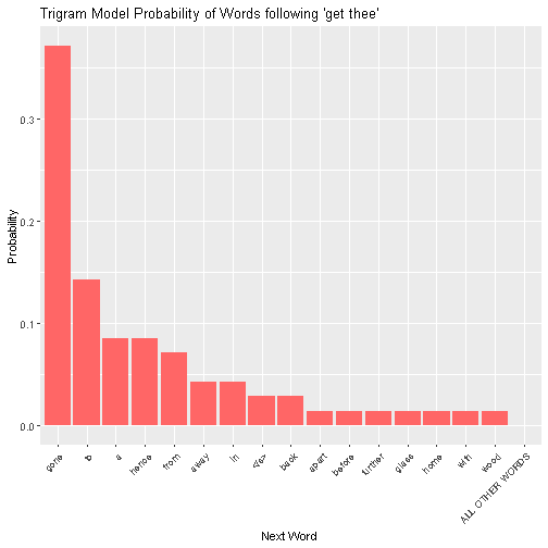 However, we want to leave room for the possibility of a word besides the 16 possibilities. That is, we want to shift some of the probability mass in the above plot to “ALL OTHER WORDS”. This means we need to determine how much probability we want to give “ALL OTHER WORDS”, and how much we should take from the other possibilities. What we are doing here “smoothing” the distribution. There are a number of schemes for smoothing. We are going to use a method called Good-Turing smoothing (yes, that guy!).
Good-Turing Smoothing
Here’s the idea. We observe there are 70 instances of ‘get thee’ in Shakespeare. In 26 of them, the next word is ‘gone’, in ten of them, the next word is ‘to’. For seven words (‘apart’, ‘before’, ‘further’, ‘glass’, ‘home’, ‘with’ and ‘wood’), the instance of “get thee” + the word is the only such instance in the whole corpus. If one was reading Shakespeare’s works start to finish (a weekend well spent), of the 70 times they read ‘get thee’, there would be 7 instances where the following word made the phrase the unique instance of that phrase in the corpus. Thus, we might estimate that the probability of seeing a new word is 7/70. Indeed, in Good-Turing smoothing, that is the probability that we would assign “ALL OTHER WORDS”. However, we need to adjust the probabilities for the other possibilities, since they need to sum to 1.
How do we do this? Consider the word ‘apart’, which appears once in our reading after ‘get thee’. What is the probability of seeing it a second time (e.g., our user entering ‘get thee apart’)? In our reading, there were two words that were such that “get thee” + the word appeared twice, namely, “back” and “”. So, if you flip to a random page and see the word “get thee”, the probability that the next word is a word that appears twice in the corpus after “get thee” is $2 \cdot \frac{2}{70} = \frac{4}{70}$. Thus, we estimate the probability of the user entering “apart”, “before”, “further”, “glass”, “home”, “with”, or “food” to be 4/70. We shall give each of these possibilities equal weight, meaning the probability of “apart” is one seventh of $\frac{4}{70}$, $\frac{2}{245}$ (this is also the probability for the other six).
How about for the word “back”? It appears twice after “get thee” in our reading, and we want to estimate the probability of seeing it a third time. In the corpus, there are 2 words that appear 3 times after “get thee”, namely, “away” and “in”. Thus, given that you see the phrase “get thee”, the probability the next word is a word that appears 3 times after “get thee” is $2 \cdot \frac{3}{70} = \frac{6}{70}$. So, we estimate the probability of a user entering “back” or “is” to be $\frac{6}{70}$. Once again, we give both equal weight, and so we set the probability of seeing “back” after “get thee” as one half of $\frac{6}{70}$, $\frac{3}{70}$.
What’s the general formula here? When we estimated the probability of seeing “back” (a word that follows “get thee” twice), we looked at the number of words that follow “get thee” 3 times (that value is 2), and multiplied by 3. This number gives the number of times, when reading the works of Shakespeare over the weekend, that you read a word that follows “get thee” which appears 3 times after “get thee” in the corpus. Dividing by 70 (the number of times “get thee” shows up at all), we get the probability of such a thing happening. Finally, we divide this value by the number of words that appear twice after “get thee” in the corpus to give equal weight to both possibilities. In our case, we divided it by 2.
To get the formula, we introduce a little notation. Let $N_c$ be the number of words that show up $c$ times after “get thee” in the corpus, and let $N$ be the number of times “get thee” shows up in the corpus. So, we have $N_1=7$, $N_2=2$, $N_3=2$, $N_{26}=1$, etc. Our calculation was then: \(P(\text{back} \mid \text{get thee}) = \frac{3N_{3}}{N N_2}\) and in general, estimated probability of a user typing a word that shows up $c$ times after “get thee” (call this value $p_c$) is: \(p_c = \frac{(c+1) N_{c+1}}{N N_c}\) This works well when $c$ is small. What about when $c=26$? There are no words that show up 27 times after “get thee”, so $N_{27}=0$, meaning $p_{26}=0$, meaning we will give a probability of $0$ to seeing “gone”, which is clearly undesirable. Indeed, this will be true for any $c$ such that there are no instances of a word following “get thee” $c+1$ times.
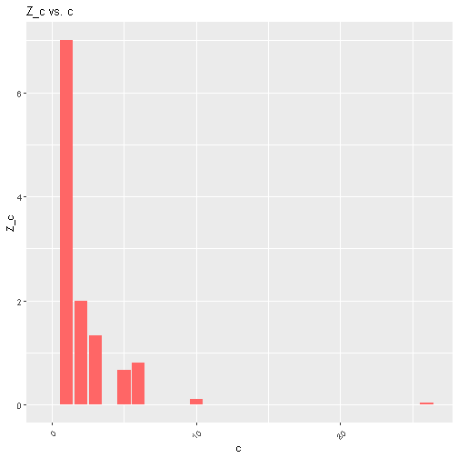
To address this, we can use approximate values for $N_c$. There are a number of ways to do this. We shall use the approach of Church and Gale (1991). Consider the frequency plot for our “get thee” example:
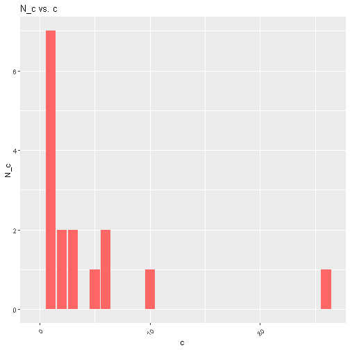 We begin by smoothing these bars. For each $c$ such that $N_c > 0$, we identify the highest $b$ such that $b < c$ and $N_b > 0$, and the smallest $d$ such that $c < d$ and $N_d > 0$. For instance, if $c=10$, then $b=6$, and $d=26$. Then, we define the approximate frequency:
\(Z_c = \frac{N_c}{0.5(d-b)}.\)
We begin by smoothing these bars. For each $c$ such that $N_c > 0$, we identify the highest $b$ such that $b < c$ and $N_b > 0$, and the smallest $d$ such that $c < d$ and $N_d > 0$. For instance, if $c=10$, then $b=6$, and $d=26$. Then, we define the approximate frequency:
\(Z_c = \frac{N_c}{0.5(d-b)}.\)
If $c=1$, we just set $N_c = Z_c$. If $c$ is the maximum, we let $d$ be such that $d - c = c - b$. The idea of this approximation is the following. Partition the $c$ axis, where splits happen at the midpoints between those $c$ for which $N_c > 0$. In our above case, these splits happen at 1.5, 2.5, 4, 5.5, 8, and 18. For each interval, we assume the value inside the split is actually evenly spread around the interval. $Z_c$ is the height of the resulting rectangle. We get the resulting plot for $Z_c$ vs $c$:
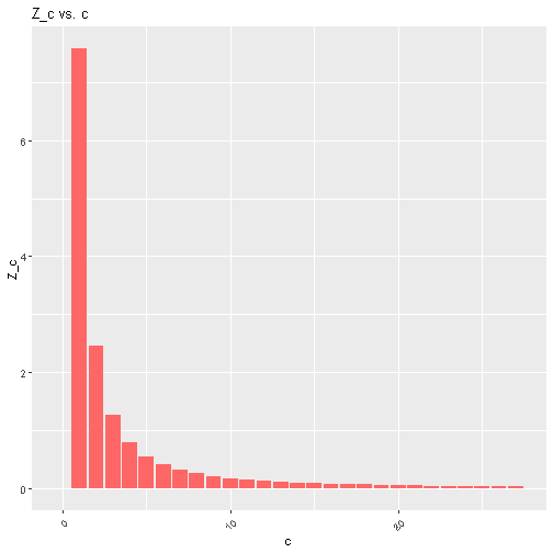
 Then, a curve is fitted to these points, by assuming a power-law relationship between $Z_c$ and $c$. That is, assuming $Z_c = Ac^B$ for some constants $A$ and $B$. This can be done by performing linear regression on the equation $\log(Z_c)= B\log{c} + \log(A)$. Using the power-law, we can then calculate this smoothed value of $Z_c$ for all $c$:
 Now we have frequencies we can use to estimate our word probabilities. Let $c(w)$ be the number of times word $w$ shows up after “get thee”. If $c(w) > 0$, the smoothed “probability” is:
\(p_s(w) = \frac{(c(w)+1)Z_{c(w)+1}}{Z_{c(w)} N},\)
and if $c(w)=0$, the value is $\frac{Z_1}{N}$. However, these aren’t true probabilities, since they don’t add up to one (this happened because we approximated with $N_c$ with $Z_c$). So, we normalize by summing up the probabilities for all words, and dividing each probability by the result. Let $c(w)$ be the number of times word $w$ shows up after “get thee”. Letting $V$ be our list of possible next words, including the catch-all bucket “ALL OTHER WORDS”, we have:
\(P_{GT}(w \mid \text{get thee}) = \frac{p_s(w)}{\sum_{w’ \in V} p_s(w’)}\)
The Good-Turing distribution then looks like the following:
Now we have frequencies we can use to estimate our word probabilities. Let $c(w)$ be the number of times word $w$ shows up after “get thee”. If $c(w) > 0$, the smoothed “probability” is:
\(p_s(w) = \frac{(c(w)+1)Z_{c(w)+1}}{Z_{c(w)} N},\)
and if $c(w)=0$, the value is $\frac{Z_1}{N}$. However, these aren’t true probabilities, since they don’t add up to one (this happened because we approximated with $N_c$ with $Z_c$). So, we normalize by summing up the probabilities for all words, and dividing each probability by the result. Let $c(w)$ be the number of times word $w$ shows up after “get thee”. Letting $V$ be our list of possible next words, including the catch-all bucket “ALL OTHER WORDS”, we have:
\(P_{GT}(w \mid \text{get thee}) = \frac{p_s(w)}{\sum_{w’ \in V} p_s(w’)}\)
The Good-Turing distribution then looks like the following:
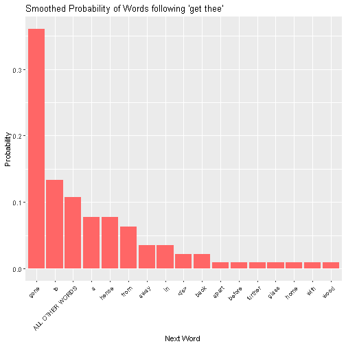 So, it looks like we leave around a 10% chance that the next word isn’t among the 16 seen in the corpus, since around 10% of the time, a word is new!
What do we do from here? We now back-off to the bigram model. We shall look at all bigrams starting with “thee” such that the second word is not among the 16 words already assigned probabilities. The remaining 10% is then proportionally split among the new options. From the bigram model, we can also back-off to a unigram model in a similar way.
Long post, but I hope this gives a good feel for how Good-Turing smoothing works for those searching!